NN-based PDE solver

Illustration of the NN-based PDE solver workflow.

Description

The high-throughput solution of PDEs for inverse modelling, design and optimization leads to requirements of very fast solutions that are largely beyond the capability of traditional PDE solver libraries.The NN-based PDE solver workflow is developed for such purpose, which could predict the full field solutions orders faster than the traditional PDE solvers. Such solver works for both small dataset, which only contains a few of BVPs, and large dataset, which could contain hundreds of thousands BVPs.

Examples

Example 1: Steady state diffusion on an octagon domain with mixed BCs

Simulation setup

Here, we use the proposed PDE constrained NNs to solve steady-state diffusion on an octagonal domain with mixed BCs, as shown in the following figure, whose solution is nonlinear in both X- and Y- directions.

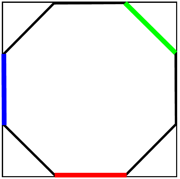
Illustration of the setup of the BVP (red: zero Dirichlet BC, green: non-zero Dirichlet BC, blue: non-zero Neumann BC).

Data preparation

Since the NN-based PDE solver only takes BCs information as inputs, the training data can be generated with any software, as long as the format is consistent as discussed in [1]. The required data for this example is provided at

ls examples/pde_solver/Example1_diffusion_steady_state/data

Configuration file

Input parameters are defined in the .ini configuration file. For deterministic NNs, the data location is given by

[NN]
DataPath = data/octagon-32x32/
DataFolder = DNS/

For small dataset, it will be augmented by 2^# times with # given at

DataAugTimes = 14

The training information is given at

Epochs = 5000
InitialEpoch = 100
BatchSize = 512
Optimizer = Nadam
LearningRate = 0.00025

where InitialEpoch refers to the zero initialization in [1].

The NN architecture is given at

NNArchitecture = 
 type=PDERandom;
 type=Conv2D | filters=8 | kernel_size=5 | activation=relu | padding=same;
 type=MaxPooling2D | pool_size=(2,2) | padding=same;
 type=Conv2D | filters=8 | kernel_size=5 | activation=relu | padding=same;
 type=MaxPooling2D | pool_size=(2,2) | padding=same;
 type=Conv2D | filters=8 | kernel_size=5 | activation=relu | padding=same;
 type=MaxPooling2D | pool_size=(2,2) | padding=same;
 type=Flatten;
 type=Dense | units=32 | activation=relu;
 type=Dense | units=32 | activation=relu;
 type=Reshape | target_shape=[4,4,2];
 type=Conv2D | filters=8 | kernel_size=5 | activation=relu | padding=same;
 type=UpSampling2D | size=(2,2);
 type=Conv2D | filters=8 | kernel_size=5 | activation=relu | padding=same;
 type=UpSampling2D | size=(2,2);
 type=Conv2D | filters=8 | kernel_size=5 | activation=relu | padding=same;
 type=UpSampling2D | size=(2,2);
 type=Conv2D | filters=8 | kernel_size=5 | activation=relu | padding=same;
 type=Conv2D | filters=1 | kernel_size=5 | activation=relu | padding=same;

which includes a list of Conv2D, MaxPooling2D, Dense, UpSampling2D layers. The PDERandom layer refers to the process where we fill random numbers to the interior region of a domain in the Dirichlet channel of augmented dataset to ensure each input is independent from each other.

For Bayesian NNs (BNN), similar as for the deterministic NNs, the data location is given by

[NN]
DataPath = data/octagon-32x32/
DataFolder = DNS/

For small dataset, it will be augmented by 2^# times with # given at

DataAugTimes = 14

The training information is given at

Epochs = 5000
InitialEpoch = 100
BatchSize = 256
MonteCarloNum = 100
Sigma1 = 1.0e-3
Sigma2 = 1.0e-2
Optimizer = Nadam
LearningRate = 2.0e-6

where InitialEpoch refers to the zero initialization in [1]. Note, if we train the BNNs with cold start, the zero initialization will play a role. If the BNNs are trained with warm start, zero initialization process will be skipped. Sigma1 is the additive noise applied to the solution. The initial value of Sigma2 is provided, which will evolve during the training.

For warm start, one needs to provide the training log file (saved as a .pickle file in the results/) to the following line.

SaveCNNModel = 

The NN architecture is given at

NNArchitecture = 
 type=PDERandom;
 type=Convolution2DFlipout | filters=8 | kernel_size=5 | activation=relu | padding=same;
 type=MaxPooling2D | pool_size=(2,2) | padding=same;
 type=Convolution2DFlipout | filters=8 | kernel_size=5 | activation=relu | padding=same;
 type=MaxPooling2D | pool_size=(2,2) | padding=same;
 type=Convolution2DFlipout | filters=8 | kernel_size=5 | activation=relu | padding=same;
 type=MaxPooling2D | pool_size=(2,2) | padding=same;
 type=Flatten;
 type=DenseFlipout | units=32 | activation=relu;
 type=DenseFlipout | units=32 | activation=relu;
 type=Reshape | target_shape=[4,4,2];
 type=Convolution2DFlipout | filters=8 | kernel_size=5 | activation=relu | padding=same;
 type=UpSampling2D | size=(2,2);
 type=Convolution2DFlipout | filters=8 | kernel_size=5 | activation=relu | padding=same;
 type=UpSampling2D | size=(2,2);
 type=Convolution2DFlipout | filters=8 | kernel_size=5 | activation=relu | padding=same;
 type=UpSampling2D | size=(2,2);
 type=Convolution2DFlipout | filters=8 | kernel_size=5 | activation=relu | padding=same;
 type=Convolution2DFlipout | filters=1 | kernel_size=5 | activation=relu | padding=same;

which includes a list of Convolution2DFlipout, MaxPooling2D, DenseFlipout, UpSampling2D layers. Again, the PDERandom layer refers to the process where we fill random numbers to the interior region of a domain in the Dirichlet channel of augmented dataset to ensure each input is independent from each other.

How to run the example

The following commands will run the deterministic NN-based PDE solver

cd examples/pde_solver/Example1_diffusion_steady_state/
python main.py octagon-32x32-cnn.ini

The simulation results will be saved in the results/ folder. The checkpoints are saved in the restart/ folder.

To run the Bayesian NN example with a warm start as discussed in [1], one need to provide the training summary pickle file from results/ to octagon-32x32-bnn.ini. The training summary file can be found from

ls results/\*.pickle

One need to edit octagon-32x32-bnn.ini

vi octagon-32x32-bnn.ini

and provide the pickle to the variable SaveCNNModel in the input file

[NN]
SaveCNNModel = results/{auto_generated_deterministic_model_summary}.pickle

Please replace {auto_generated_deterministic_model_summary} with the actual name of the pickle file.

Following that step, one can run the probabilistic NN-based PDE solver via

python main.py octagon-32x32-bnn.ini

Results

At the end of training, the NN-based PDE solver will output training loss and NN predicted results for one testing data point in the “results/” folder.

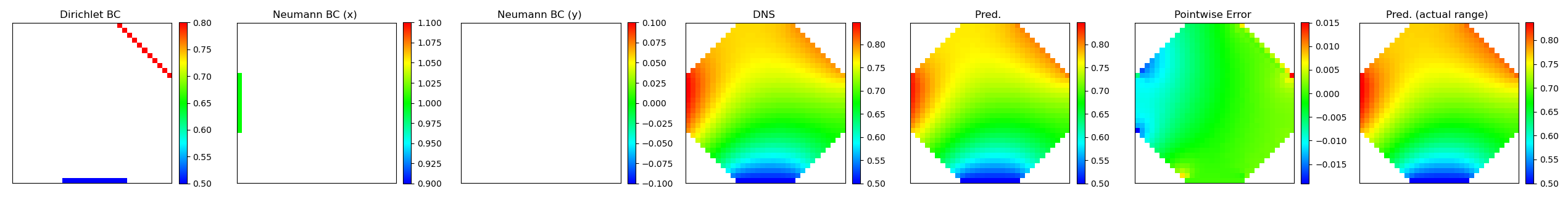
Results: 1. Dirichlet BC, 2. Neumann BC in x direction, 3. Neumann BC in y direction, 4. DNS solution, 5. NN predicted results (determnistic) or mean of NN predicted results (Bayesian) with the same color legend as 4, 6. Pointwise error between 4 and 5, 7. similar as 5 but with a color legend representing the actual predicted solution range.

Example 2: Linear elasticity on a square domain with Dirichlet BCs

Simulation setup

Here, we use the proposed PDE constrained NNs to solve linear elasticity on a square domain with Dirichlet BCs, as shown in the following figure, whose solution is nonlinear in both X- and Y- directions.

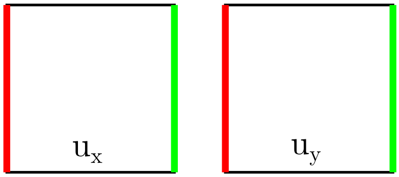
Illustration of the setup of the BVP (red: zero Dirichlet BC, green: non-zero Dirichlet BC).

Data preparation

Since the NN-based PDE solver only takes BCs information as inputs, the training data can be generated with any software, as long as the format is consistent as discussed in [1]. The required data for this example is provided at

ls examples/pde_solver/Example2_linear_elasticity/data

Configuration file

Similar as example 1

How to run the example

Similar as example 1

Results

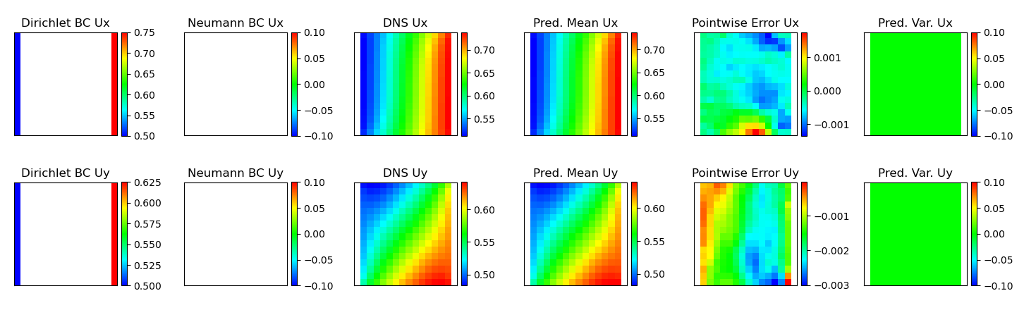
At the end of training, the NN-based PDE solver will output training loss and NN predicted results for one testing data point in the “results/” folder.

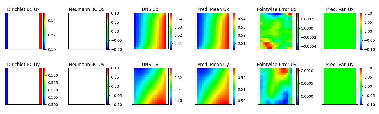
Results: 1. Dirichlet BC, 2. Neumann BC, 3. DNS solution, 4. NN predicted results (determnistic) or mean of NN predicted results (Bayesian) with the same color legend as 3, 5. Pointwise error between 3 and 4, 6. Predicted variance for Bayesian NNs (zero for deterministic NNs).

Example 3: Non-linear elasticity on a square domain with Dirichlet BCs

Simulation setup

Here, we use the proposed PDE constrained NNs to solve nonlinear elasticity on a square domain with Dirichlet BCs, as shown in the following figure, whose solution is nonlinear in both X- and Y- directions.

Illustration of the setup of the BVP (red: zero Dirichlet BC, green: non-zero Dirichlet BC).

Data preparation

Since the NN-based PDE solver only takes BCs information as inputs, the training data can be generated with any software, as long as the format is consistent as discussed in [1]. The required data for this example is provided at

ls examples/pde_solver/Example3_nonlinear_elasticity/data

Configuration file

Similar as example 1

How to run the example

Similar as example 1

Results

At the end of training, the NN-based PDE solver will output training loss and NN predicted results for one testing data point in the “results/” folder.

Results: 1. Dirichlet BC, 2. Neumann BC, 3. DNS solution, 4. NN predicted results (determnistic) or mean of NN predicted results (Bayesian) with the same color legend as 3, 5. Pointwise error between 3 and 4, 6. Predicted variance for Bayesian NNs (zero for deterministic NNs).

Remarks

Command line

How to restart simulation from a specific check point (e.g. epoch 5000) and make predictions

cd examples/pde_solver/Example1_diffusion_steady_state/
python main.py octagon-32x32-cnn.ini -rf results/{auto_generated_model_summary}.pickle -ra 5000

If the option “-ra” is not provided, the simulation will restart from the latest check point.

How to restart simulation from a specific check point and continue running the problem for another 1000 epochs

cd examples/pde_solver/Example1_diffusion_steady_state/
python main.py octagon-32x32-cnn.ini -rf results/{auto_generated_model_summary}.pickle -c 1000

Note

Tensorflow and tensorflow-probability libraries installed by the requirements.txt are CPU-based distributions. If you have a CUDA-enabled machine, you can also install the GPU versions of these two libraries to speedup the training. In general, tensorflow version needs to be greater than 2.2. The version of tensorflow-probability needs to be compatible with the version of tensorflow. This is automatically handled by the provided installation instructions.

References

[1]. X Zhang, K Garikipati. “Bayesian neural networks for weak solution of PDEs with uncertainty quantification”, preprint at arXiv:2101.04879.