Active learning
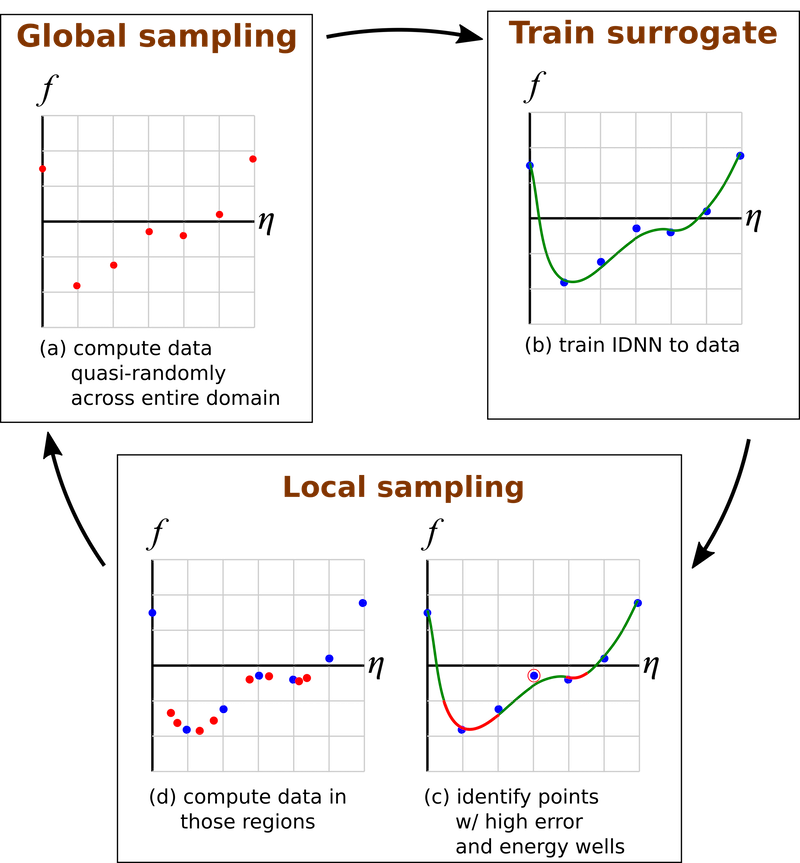
Schematic of the active learning workflow for learning free energy density function.
Description
The active learning workflow combines global and local sampling to create a well-sampled dataset with a corresponding surrogate model.
Examples
Example1: Learning free energy density for scale bringing: Ni-Al system
This example manages the creation of a free energy density function for the Ni-Al system, where the data are found using Monte Carlo simulations based on statistical mechanics, using in-house versions of the CASM software [github.com/prisms-center/CASMcode]. The surrogate model is an integrable deep neural network (IDNN).
The following python class defines the active learning workflow for the Ni-Al free energy project. First, the class constructor, which sets up necessary directories and defines an initial IDNN (other IDNNs will also be created later on, at each iteration of the workflow).
    def __init__(self,config_path,test=False):

        self.test = test

        if not os.path.exists('training'):
            os.mkdir('training')
        if not os.path.exists('data'):
            os.mkdir('data')
        if not os.path.exists('outputFiles'):
            os.mkdir('outputFiles')

        self.read_config(config_path)
        self.seed = 1 # initial Sobol sequence seed

        # initialize IDNN
        self.hidden_units = [20,20]
        self.lr = 0.2
        self.idnn = IDNN(self.dim,
                         self.hidden_units,
                         transforms=self.IDNN_transforms(),
                         dropout=self.Dropout,
                         unique_inputs=True,
                         final_bias=True)
        self.idnn.compile(loss=['mse','mse',None],
                          loss_weights=[0.01,1,None],
                          optimizer=keras.optimizers.Adagrad(lr=self.lr))
Next, we read in the parameters defined in the configuration file, such as the number of workflow iterations, the number of CPUs to use for the direct numerical simulations, the number of hyperparameter sets to compare, etc.
    def read_config(self,config_path):

        config = ConfigParser()
        config.read(config_path)

        self.casm_project_dir = config['DNS']['CASM_project_dir']
        self.job_manager = config['DNS']['JOB_MANAGER']
        self.N_jobs = int(config['HPC']['CPUNum']) #number of processors to use
        self.N_global_pts = int(config['WORKFLOW']['N_global_pts']) #global sampling points each iteration
        self.N_rnds = int(config['WORKFLOW']['Iterations'])
        self.Epochs = int(config['NN']['Epochs'])
        self.Batch_size = int(config['NN']['Batch_size'])
        self.N_hp_sets = int(config['HYPERPARAMETERS']['N_sets'])
        self.Dropout = float(config['HYPERPARAMETERS']['Dropout'])
        self.dim = 4
        if self.job_manager == 'PC' and self.N_jobs > 1:
            self.N_jobs = 1
            self.casm_project_dir = '.'
            print("WARNING: only one processor is allowed for running on your personal computer; CPUNum is overridden by 1")
The following function defines a test set, or a sample set. Here, points are first sampled from the sublattice composition space, since the bounds are well-defined: [0,1]. Sampling is done with a Sobol sequence because if its space-filling and noncollapsing design. These values are then converted from sublattice compositions to order parameters through a linear operation. Finally, only points with average composition less than or equal to 0.25 are taken, since the crystal structure changes from FCC to BCC at that point.
    def create_test_set(self,N_points,dim,bounds=[0.,1.],seed=1):

        Q = 0.25*np.array([[1, 1, 1, 1],
                           [1, 1, -1, -1],
                           [1, -1, -1, 1],
                           [1, -1, 1, -1]])

        # Create test set
        x_test = np.zeros((N_points,dim))
        eta = np.zeros((N_points,dim))
        i = 0
        while (i < N_points):
            x_test[i],seed = i4_sobol(dim,seed)
            x_test[i] = (bounds[1] - bounds[0])*x_test[i] + bounds[0] # shift/scale according to bounds
            eta[i] = np.dot(x_test[i],Q.T).astype(np.float32)
            if eta[i,0] <= 0.25:
                i += 1

        return x_test, eta, seed
At each iteration of the workflow, an approximation of the free energy and the chemical potential are needed. For the first iteration before any data have been computed, we use the free energy of an ideal solution. For subsequent iterations, the current IDNN is used.
    def ideal(self,x_test):

        T = 600.
        kB = 8.61733e-5
        Q = 0.25*np.array([[1, 1, 1, 1],
                           [1, 1, -1, -1],
                           [1, -1, -1, 1],
                           [1, -1, 1, -1]])
        invQ = np.linalg.inv(Q)

        g_test = 0.25*kB*T*np.sum((x_test*np.log(x_test) + (1.-x_test)*np.log(1.-x_test)),axis=1)
        mu_test = 0.25*kB*T*np.log(x_test/(1.-x_test)).dot(invQ)

        return mu_test, g_test
The active learning workflow consists of alternating between global and local sampling of the composition/order parameter space. Global sampling uses the create_test_set function defined previously to sample across the full domain, then submitting these points to the CASM code to compute the chemical potentials and order parameters.
    def global_sampling(self,rnd):

        # sample with sobol
        if rnd==0:
            x_bounds = [1.e-5,1-1.e-5]
        elif rnd<11:
            x_bounds = [-0.05,1.05]
        else:
            #x_bounds = [-0.02,1.02]
            x_bounds = [0.,1.]
        x_test,eta,self.seed = self.create_test_set(self.N_global_pts,
                                                    self.dim,
                                                    bounds=x_bounds,
                                                    seed=self.seed)

        # approximate mu
        if rnd==0:
            mu_test,_ = self.ideal(x_test)
        else:
            mu_test = 0.01*self.idnn.predict([eta,eta,eta])[1]

        # submit casm
        submitCASM(self.N_jobs,mu_test,eta,rnd,casm_project_dir=self.casm_project_dir,test=self.test,job_manager=self.job_manager)
        compileCASMOutput(rnd)
Local sampling is based on two characteristics: areas with large pointwise error and areas with local energy wells. The pointwise error is calculated for all data points from the most recent global sampling and is defined at each point as the square of the difference between the predicted and the actual chemical potential values, summed across all four chemical potentials. All these points are sorted according to the error. For each of the N (e.g. 200) points with the highest error, n (e.g. 4) random perturbations of the point are selected to be computed with CASM. This is repeated, with a lower value of n, for the next N points in the sorted list. By sampling in regions with high IDNN error, we can more rapidly improve the overall error in the IDNN.
Local energy wells define areas of phase stability. For this reason, local wells are identified and additional sampling takes place there. To do this, a large set of points are sampled across the full domain, using a Sobol sequence. The current IDNN is used to determine if each point is in a region of convexity (a potential well). For each point, the norm of the gradient also computed. The points are sorted by the norm of the gradient, since the points nearest to the minium of the well with have the lowest gradient norm. The M points in a region of convexity that have the lowest gradient norm are used to defined M*n additional sampling points, through random perturbation.
    def local_sampling(self,rnd):

        # local error
        eta_test, mu_test = loadCASMOutput(rnd-1,singleRnd=True)
        mu_pred = 0.01*self.idnn.predict([eta_test,eta_test,eta_test])[1]
        error = np.sum((mu_pred - mu_test)**2,axis=1)
        etaE =  eta_test[np.argsort(error)[::-1]]

        # find wells
        _,eta_test,self.seed = self.create_test_set(30*self.N_global_pts,
                                                    self.dim,
                                                    seed=self.seed)
        etaW = find_wells(self.idnn,eta_test)

        # randomly perturbed samples
        eta_a = np.repeat(etaE[:200],4,axis=0)
        eta_b = np.repeat(etaE[200:400],2,axis=0)
        eta_c = np.repeat(etaW[:400],4,axis=0)
        if self.test:
            eta_a = np.repeat(etaE[:2],3,axis=0)
            eta_b = np.repeat(etaE[2:4],2,axis=0)
            eta_c = np.repeat(etaW[:4],3,axis=0)
        eta_local = np.vstack((eta_a,eta_b,eta_c))
        eta_local += 0.25*(1.5/(2.*self.N_global_pts**(1./self.dim)))*(np.random.rand(*eta_local.shape)-0.5) #perturb points randomly
        mu_local = 0.01*self.idnn.predict([eta_local,eta_local,eta_local])[1]

        # submit casm
        submitCASM(self.N_jobs,mu_local,eta_local,rnd,casm_project_dir=self.casm_project_dir,test=self.test,job_manager=self.job_manager)
        compileCASMOutput(rnd)
A hyperparameter search is performed to improve training.
    def hyperparameter_search(self,rnd):
        # submit
        self.hidden_units, self.lr = hyperparameterSearch(rnd,self.N_hp_sets,job_manager=self.job_manager)
The free energy of this system is known, due to crystal symmetries, to be invariant to certain transformations of the order parameters. Those transformations are defined here, and the IDNN then becomes of a function of these transformations. In this way, the known symmetries are built in exactly.
    def IDNN_transforms(self):

        def transforms(x):
            h0 = x[:,0]
            h1 = 16.*x[:,1]*x[:,2]*x[:,3]
            h2 = 4.*(x[:,1]*x[:,1] + x[:,2]*x[:,2] + x[:,3]*x[:,3])
            h3 = 64.*(x[:,2]*x[:,2]*x[:,3]*x[:,3] +
                      x[:,1]*x[:,1]*x[:,3]*x[:,3] +
                      x[:,1]*x[:,1]*x[:,2]*x[:,2])

            return [h0,h1,h2,h3]

        return transforms
This function defines the training of the IDNN. Note that we receive DNS data for the four chemical potentials, which are the partial derivatives of the free energy with respect to the four order parameters. Since we only have derivative data, we will have an arbitrary constant of integration. While this is not a huge problem, it is inconvenient. To remedy this, we will also create free energy data that (somewhat arbitratily) defines the free energy to be zero when all order parameters are zero. (Because of the way the neural network code is defined, the number of free energy points has to be the same as the number of chemical potential points, but they do not have to be defined at the same order parameter values.) A snapshot of the IDNN with its current weights is saved at each workflow iteration.
    def surrogate_training(self,rnd):
        # read in casm data
        eta_train, mu_train = loadCASMOutput(rnd)

        # shuffle the training set (otherwise, the most recent results
        # will be put in the validation set by Keras)
        inds = np.arange(eta_train.shape[0])
        np.random.shuffle(inds)
        eta_train = eta_train[inds]
        mu_train = mu_train[inds]

        # create energy dataset (zero energy at origin)
        eta_train0 = np.zeros(eta_train.shape)
        g_train0 = np.zeros((eta_train.shape[0],1))

        # train
        lr_decay = 0.9**rnd
        self.idnn.compile(loss=['mse','mse',None],
                          loss_weights=[0.01,1,None],
                          optimizer=keras.optimizers.Adagrad(lr=self.lr*lr_decay))
        csv_logger = CSVLogger('training/training_{}.txt'.format(rnd),append=True)
        reduceOnPlateau = ReduceLROnPlateau(factor=0.5,patience=100,min_lr=1.e-4)
        earlyStopping = EarlyStopping(patience=150)
        self.idnn.fit([eta_train0,eta_train,0*eta_train],
                      [100.*g_train0,100.*mu_train,0*mu_train],
                      validation_split=0.25,
                      epochs=self.Epochs,
                      batch_size=self.Batch_size,
                      callbacks=[csv_logger,
                                 reduceOnPlateau,
                                 earlyStopping])
        self.idnn.save('idnn_{}'.format(rnd))
The main_workflow function is fairly simple, but it defines the overall workflow. Again, it begines with the global sampling. After these points are calculated through CASM, and IDNN is trained to all calculated data, including data from previous iterations. (On the second iteration of the workflow, a hyperparameter search is performed first to determine the size of the IDNN and a good value for the learning rate.) Once trained, the current IDNN is used to perform local sampling, which completes the workflow iteration. Currently, the number of iterations is given directly, but a stopping condition could be defined based on the overall change in the IDNN from one iteration to the next.
    def main_workflow(self):
        """
        Main function outlining the workflow.

        - Global sampling

        - Surrogate training (including hyperparameter search)

        - Local sampling
        """

        for rnd in range(self.N_rnds):
            self.global_sampling(2*rnd)

            if rnd==1:
                self.hyperparameter_search(rnd)
                custom_objects = {'Transform': Transform(self.IDNN_transforms())}

                unique_inputs = self.idnn.unique_inputs
                self.idnn = keras.models.load_model('idnn_1',
                                                    custom_objects=custom_objects)
                self.idnn.unique_inputs = unique_inputs

            self.surrogate_training(rnd)
            self.local_sampling(2*rnd+1)
Data preparation
Configuration file
Standard parameters in the workflow can be defined in the .ini configuration file.
The deep numerical simlation (DNS) and high performance computing (HPC) settings can be defined here, including the DNS model and any addition parameters required by the model:
[DNS]
MODEL = CASM
CASM_project_dir = ~/CASM_sampling/FCC/vcgcmc_test
JOB_MANAGER = LSF

[HPC]
CPUNum = 300
Next, define parameters related to the neural network surrogate model:
[NN]
Epochs = 600
Batch_size = 100

[HYPERPARAMETERS]
N_sets = 30
LearningRate = 0.001,0.5
Layers = 2,2
Neurons = 20,200
Dropout = 0.06
Finally, there are additional parameters specific to the active learning workflow itself:
[WORKFLOW]
Iterations = 20
N_global_pts = 1200
References
G.H. Teichert, A.R. Natarajan, A. Van der Ven, K. Garikipati. “Machine learning materials physics: Integrable deep neural networks enable scale bridging by learning free energy functions,” Computer Methods in Applied Mechanics and Engineering. Vol 353, 201-216, 2019, doi:10.1016/j.cma.2019.05.019
G.H. Teichert, A.R. Natarajan, A. Van der Ven, K. Garikipati. “Active learning workflows and integrable deep neural networks for representing the free energy functions of alloys,” Computer Methods in Applied Mechanics and Engineering. Vol 371, 113281, 2020, doi:10.1016/j.cma.2020.113281
G.H. Teichert, S. Das, M. Aykol, C. Gopal, V. Gavini, K. Garikipati. “LixCoO2 phase stability studied by machine learning-enabled scale bridging between electronic structure, statistical mechanics and phase field theories,” arXiv preprint: arxiv.org/abs/2104.08318